45 repeat item labels in a pivottable report excel 2007

(Archives) Microsoft Excel 2007: Working with PivotTables Mac - UWEC Select a cell within the data range for which you are creating a PivotTable. From the Data menu, select PivotTable Report... The PivotTable Wizard appears. Select Microsoft Excel list or database. Click Next. The PivotTable Wizard - Step 2 of 3 dialog box appears. In the Range text box, verify that your data range is indicated. OR PDF Excel Troubleshooting Row Labels in Pivot Tables You simply choose Repeat All Item Labels from the Report Layout drop-down menu. Filling in the Outline View in Excel 2007 and Earlier In Excel 2007 and earlier, you had to follow these steps: 1. Select the entire pivot table. 2. Copy the pivot table to the clipboard. 3. Use the Paste Special dialog to paste just the Values.

How to use pivot tables in excel for human resources - edubetta Then go to click Report Layout again to click Repeat All Item Labels from the list. Then click at any cell of the new pivot table, and go to the Design tab to click Report Layout > Show in Tabular Form.ġ0. Then a PivotTable Field List pane appears, and drag the Row and Column fields to the Row Labels section, and Value field to Values section.

Repeat item labels in a pivottable report excel 2007

Excel Pivot Table Report Filter Tips and Tricks To use a pivot table field as a Report Filter, follow these steps. In the PivotTable Field list, click on the field that you want to use as a Report Filter. Drag the field into the Filters box, as shown in the screen shot below. On the worksheet, Excel adds the selected field to the top of the pivot table, with the item (All) showing. How to make row labels on same line in pivot table? Please do as follows: 1. Click any cell in your pivot table, and the PivotTable Tools tab will be displayed. 2. Under the PivotTable Tools tab, click Design > Report Layout > Show in Tabular Form, see screenshot: 3. And now, the row labels in the pivot table have been placed side by side at once, see screenshot: How to Resolve Duplicate Data within Excel Pivot Tables Excel 2007 and later: As shown in Figure 2, click on cell A1, choose Insert, Table, and then click OK. Click Summarize with Pivot Table from the Design tab, and then click OK. Excel 2003 and earlier: Choose Data, List, Create, and then click OK. Next, choose Data, Pivot Table Wizard, and then click Finish. Figure 2: Carry out the steps shown to ...

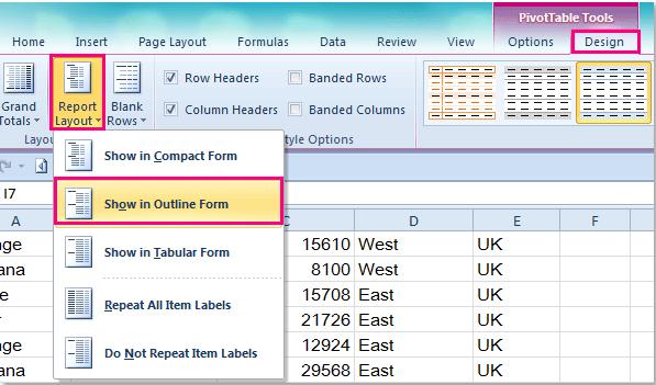
Repeat item labels in a pivottable report excel 2007. Excel Pivot Table Report - Sort Data in Row & Column Labels & in Values ... (i) manual: by choosing this option - (a) you can drag items to rearrange them the way you want - to drag, select an item and move your mouse cursor on its borders till a four-pointed arrow is formed and then hold and drag (refer image 3 to see how the arrow appears); or (b) select an item in the pivot table report and type in exactly the other … Excel Pivot Table Report Layout - Contextures Excel Tips Follow these steps, to change the layout: Select a cell in the pivot table. On the Ribbon, click the Design tab. In some versions of Excel, Design is under the PivotTable Tools tab. At the left, in the Layout group, click the Report Layout command. Click the layout that you want to uses, e.g. Show in Outline Form. PivotTable Excel 2010 (Report Layout, Repeat All Item Labels) De la versiunea Excel 2010, un tabel de tip PivotTable se poate folosi ca sursa de date. Folosim optiunea Repeat All Item Labels. Pentru a Putea folosi optiunea "Repeat All Item Labels" clic pe PivotTable Tools Design (pasul 1), Clic Report Layout ( pasul 2), Clic Repeat All Item Labels (pasul 3) Repeat row labels in a PivotTable - Microsoft Community Excel; Microsoft 365 and Office; Search Community member; pbgarcia. Created on January 9, 2012. Repeat row labels in a PivotTable Hello all, I have the following PiovtTable: Sum of Amt Billed: CLARK: 200 $ ... Excel 2010 introduces the Report Layout > Repeat All Item Labels feature.

› excel-pivot-tables › how-to-useHow to Use Pivot Table Field Settings and Value ... - Excel Tip You can choose to show items in tabular format or not, choose to repeat item labels or not. Choose to insert a blank line after each item label or not. Choose to show items with no data or not. So yeah, this is how you can access field settings and value field settings in Excel Pivot Tables. I hope this helped you. How to repeat row labels for group in pivot table? - ExtendOffice In the Field Settings dialog box, click Layout & Print tab, then check Repeat item labels, see screenshot: 4. And then click OK to close the dialog, and now, you can see the row labels which you have specified are repeated only. How to create clickable hyperlinks in pivot table? How to display grand total at top in pivot table? Value filter in pivot tabel (Office 2007) - MrExcel Message Board May 26, 2011. #26. Reply is a bit late, i know, but i was just trying to find this out myself. Found this in the help file on pivottables: You cannot filter by label, date or time, value, or top or bottom numbers if the PivotTable data source is an OLAP database that does not support the MDX expression subselect syntax. Repeating Attribute Names in Excel - social.msdn.microsoft.com In Excel .. cell Country right-click and choose Field Settings from the context menu. In tab Layout & Print check Repeat item labels. Marco Schreuder IN2BI DWH Deck

Repeat Pivot Table Labels in Excel 2010 Right-click one of the Region labels, and click Field Settings In the Field Settings dialog box, click the Layout & Print tab Add a check mark to Repeat item labels, then click OK Now, the Region labels are repeated, but the City labels are only listed once. Watch the Pivot Table Repeat Labels Video Spreadsheets: Problems with Pivot Table Labels - CFO To return to a normal layout of the pivot table, follow these steps: 1. Select any cell inside the pivot table. The PivotTable Tools tabs appear in the Ribbon. 2. Go to Design tab of the ribbon. 3. From the Design tab, open the Report Layout dropdown. 4. Choose Show in Tabular Form as shown in Figure 2. Fig. 2 Excel For Mac Pivot Table Repeat Item Labels - truehfil You can then select to Repeat All Item Labels which will fill in any gaps and allow you to take the data of the Pivot Table to a new location for further analysis. Right-click the row or column label you want to repeat, and click Field Settings. Click the Layout & Print tab, and check the Repeat item labels box. Option to group repeating cells in reports produced in Excel 2007 format By default, repeating cells are merged in Excel 2007 output. For example, Product line is a grouped column in a list. The values for Product line, such as Camping Equipment and Golf Equipment, appear once in a merged cell in Excel output. When repeating cells are not grouped, the values for Product line appear in each repeating cell.

How to repeat row labels for group in pivot table?

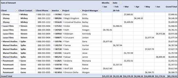
How To Format Excel PivotTables For Even Greater Effect To turn on the Repeat All Item Labels, again return to the PivotTable Design tab of the Ribbon. Then click Report Layout, followed by Repeat All Item Labels. As Figure 5 shows, this action fills the data in the Client, Client Contact, and Client Phone fields of the PivotTable, creating a format that many will find familiar.

How to reverse a pivot table in Excel?

Repeating Values in Pivot Tables - Daily Dose of Excel To do that, I first go to the PivotTable Options - Display tab and change it to Classic PivotTable layout. Then I'll go to each PivotItem that's a row and remove the subtotal and check the Repeat item labels checkbox. And I get a PivotTable that's ready for copying and pasting. After about 50 times of doing that, I got sick of it.

How To Format Excel PivotTables For Even Greater Effect - K2 Enterprises

› charts › panel-templateHow to Create a Panel Chart in Excel – Automate Excel Choose “PivotTable.” When the Create PivotTable dialog box appears, select “Existing Worksheet,” highlight any empty cell near your actual data (G1), and click “OK.” Step #3: Design the layout of the pivot table. Immediately after your pivot table has been created, the PivotTable Fields task pane will pop up. In this task pane ...

Share :