39 conditional formatting data labels excel
How to Create Excel Charts (Column or Bar) with Conditional Formatting ... Conditional formatting is the practice of assigning custom formatting to Excel cells—color, font, etc.—based on the specified criteria (conditions). The feature helps in analyzing data, finding statistically significant values, and identifying patterns within a given dataset. How to Use Conditional Formatting Based on Date in Microsoft Excel Open the sheet, select the cells you want to format, and head to the Home tab. In the Styles section of the ribbon, click the drop-down arrow for Conditional Formatting. Move your cursor to Highlight Cell Rules and choose "A Date Occurring" in the pop-out menu. A small window appears for you to set up your rule.
Conditional formatting with formulas (10 examples) | Exceljet You can create a formula-based conditional formatting rule in four easy steps: 1. Select the cells you want to format. 2. Create a conditional formatting rule, and select the Formula option 3. Enter a formula that returns TRUE or FALSE. 4. Set formatting options and save the rule.

Conditional formatting data labels excel
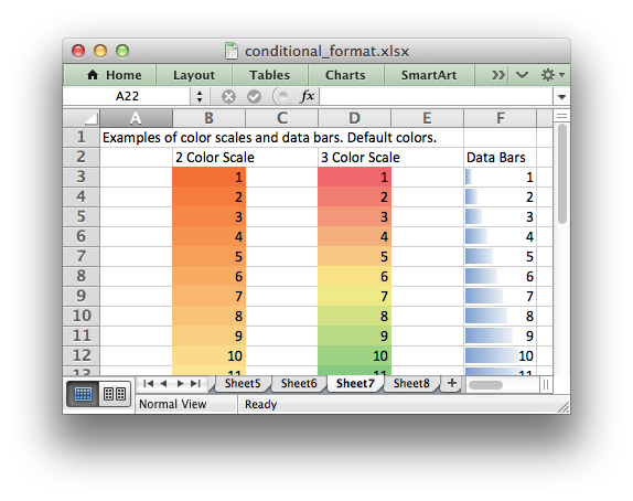
Format Data Labels in Excel- Instructions - TeachUcomp, Inc. To format data labels in Excel, choose the set of data labels to format. To do this, click the "Format" tab within the "Chart Tools" contextual tab in the Ribbon. Then select the data labels to format from the "Chart Elements" drop-down in the "Current Selection" button group. VBA Conditional Formatting of Charts by Value and Label The category labels (XValues) and values (Values) are put into arrays, also for ease of processing. The code then looks at each point's value and label, to determine which cell has the desired formatting. The rows and columns are looped starting at 2, since the first of each contains an irrelevant label. The looping stops one count before the end. Excel conditional formatting Icon Sets, Data Bars and Color Scales Select all cells in column A, except for the column header, and create a conditional formatting icon set rule by clicking Conditional Formatting > Icon sets > More Rules... In the New Formatting Rule dialog, select the following options: Click the Reverse Icon Order button to change the icons' order. Select the Icon Set Only checkbox.
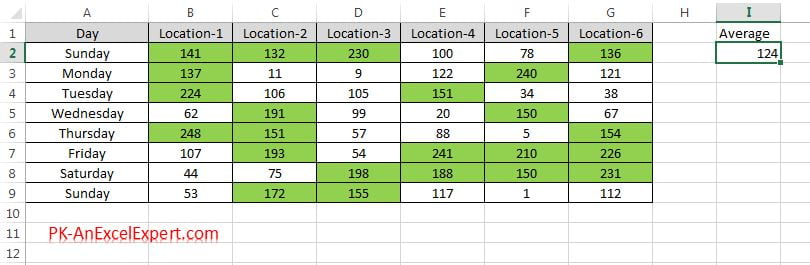
Conditional formatting data labels excel. How to do conditional formatting of a label in Excel VBA Function ConditionalFormatNumber (n As Double) As String If n > 1000000 Then ConditionalFormatNumber = Format (n / 1000000, "$#,##0.00,,""M""") ElseIf n > 1000 Then ConditionalFormatNumber = Format (n / 1000, "$#,##0.00, ""K""") Else ConditionalFormatNumber = Format (n, "$#,##0.0") End If End Function Share answered Aug 24, 2017 at 9:13 Change the format of data labels in a chart To get there, after adding your data labels, select the data label to format, and then click Chart Elements > Data Labels > More Options. To go to the appropriate area, click one of the four icons ( Fill & Line, Effects, Size & Properties ( Layout & Properties in Outlook or Word), or Label Options) shown here. Excel Conditional Number Formatting In Charts - Stack Overflow I am working with Excel 2010 and I want to apply conditional number formatting to value labels in a chart. When I apply the conditional formatting to the cells within the workbook, the conditional formatting works just fine, but when I feed that data to a chart the conditional number formatting is lost on the value labels. Excel Data Analysis - Conditional Formatting - tutorialspoint.com Follow the steps to conditionally format cells − Select the range to be conditionally formatted. Click Conditional Formatting in the Styles group under Home tab. Click Highlight Cells Rules from the drop-down menu. Click Greater Than and specify >750. Choose green color. Click Less Than and specify < 500. Choose red color.
Custom Chart Data Labels In Excel With Formulas - How To Excel At Excel Follow the steps below to create the custom data labels. Select the chart label you want to change. In the formula-bar hit = (equals), select the cell reference containing your chart label's data. In this case, the first label is in cell E2. Finally, repeat for all your chart laebls. Conditional Formatting Shapes - Step by step Tutorial Let's see step by step how to create it: First, select an already formatted cell. In the picture below, we have created a little example of this. We will pay attention to the range D5:D6. You can see the rules in the Rules Manager window. We didn't make it overly complicated. Changing the Color of a Data Label using IF Statement 1) Click on the data labels to highlight all the data labels, 2) Right-Click and select Format Data Labels, 3) Click on Number, 4) Go to the Format Code field *adapt the following to your needs* 5) [green] [>29]#.00; [<30] [Color 53]#.00 Click to expand... Hi Jawnne, I hope you're still lurking about on here. Custom Data Labels with Colors and Symbols in Excel Charts - [How To ... To apply custom format on data labels inside charts via custom number formatting, the data labels must be based on values. You have several options like series name, value from cells, category name. But it has to be values otherwise colors won't appear. Symbols issue is quite beyond me.
Conditional Formatting with Data Validation - Microsoft Tech Community For example, if A2=Value, B2= Value, and C2 is blank, I would like to have C2 turn red. A2,B2, and C2 all have a list range for the Data Validation. For the conditional formatting, I have only put the range to apply to as column C. The conditional formatting is not turning cells red as needed. I am not sure what the issue is. How to change chart axis labels' font color and size in Excel? Sometimes, you may want to change labels' font color by positive/negative/ in an axis in chart. You can get it done with conditional formatting easily as follows: 1. Right click the axis you will change labels by positive/negative/0, and select the Format Axis from right-clicking menu. 2. Excel Conditional Formatting Data Bars - Contextures Excel Tips On the Ribbon, click the Home tab. In the Styles group, click Conditional Formatting, and then click Manage Rules. In the list of rules, click your Data Bar rule. Click the Edit Rule button, to open the Edit Formatting Rule dialog box. In the second section -- Edit the Rule Description -- add a check mark to Show Bar Only. Use conditional formatting to highlight information On the Home tab, in the Styles group, click the arrow next to Conditional Formatting, and then click Manage Rules. The Conditional Formatting Rules Manager dialog box appears. The conditional formatting rules for the current selection are displayed, including the rule type, the format, the range of cells the rule applies to, and the Stop If True setting.
How to train your users to create their own Business Intelligence reports? #4 of 5: Sample ...
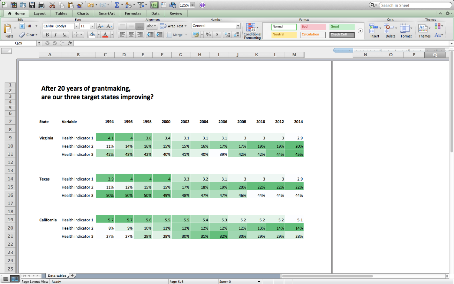
Conditional Formatting in Excel - Endsight First, highlight the values that we want formatted. Go to the Home tab, under the Styles section, and click Conditional Formatting. Excel has a variety of pre-set templates with rules for highlighting particular cell ranges, adding bars based on values, color scales, and even icons. Feel free to explore these different template rules.
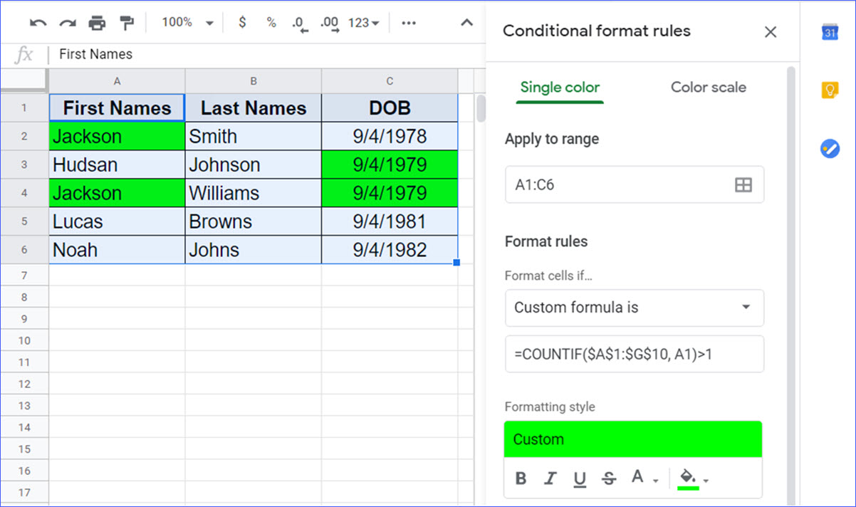
How to Highlight Duplicates in Google Sheets - ExcelNotes
Conditional formatting shortcut - Excel Hack Excel's conditional formatting is a tool that allows you to apply any formatting to cells that meet certain conditions. For example, you can apply a format that is useful for managing data, such as highlighting cells with a number greater than 50. Below is a shortcut that will help you use conditional formatting more quickly.

How to use Conditional Formatting in Excel (15 awesome tricks)
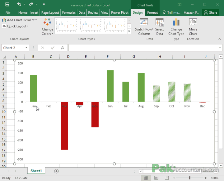
Conditional formatting for Excel column charts Initial formatting. The initial chart looks strange because for each month there is room for four columns but only one of the columns is showing. Click on one of the columns. Press Ctrl+1 to open the Format Data Series task pane. Set the Series Overlap to 100% and the Gap Width to 50%. The Series Overlap layers the columns on top of each other ...

How to Create Multi-Category Chart in Excel - Excel Board
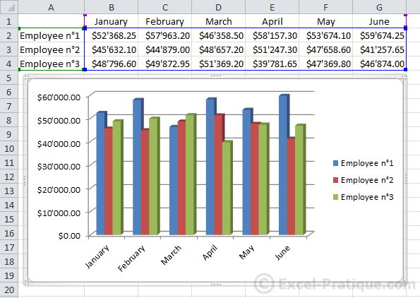
Excel tutorial: How to use data labels Generally, the easiest way to show data labels to use the chart elements menu. When you check the box, you'll see data labels appear in the chart. If you have more than one data series, you can select a series first, then turn on data labels for that series only. You can even select a single bar, and show just one data label.
SQL Workbench/J User's Manual SQLWorkbench
Conditional format of chart labels - Excel Help Forum Whilst Conditional Formatting will not be pickup by the data labels there may be alternative approaches before reverting to VBA. Custom number format could control colour. Additional series in the chart could provide differently formatted labels. Can you post example and detail of what the CF is. Cheers Andy Register To Reply
Moving X-axis labels at the bottom of the chart below negative values in Excel - PakAccountants.com
Conditional Formatting in Excel - a Beginner's Guide - GoSkills.com Click Conditional Formatting, then select Icon Set to choose from various shapes to help label your data. For this example, let's use the arrow icon set to show whether our highlighted data, the Variance column, has increased or decreased. Now, you'll see that the data has arrow icons accompanying their values in the cells.
Excel Course: Inserting Graphs
Conditional Formatting to Distinguish Between Labels and Numbers I want to conditionally format each cell, so that the text is yellow, the numbers are blue, and the blank cells are green. I tried by setting up a new rule under conditional formatting, then selecting "use a formula to determine which cells to format", then using some combinations of the if, istext, isnumber, etc. combinations. Please advise.

How to use Conditional Formatting in Excel? - GeeksforGeeks
Conditional Formatting in Excel (Complete Guide + Examples) Select the Home tab's Conditional Formatting icon in the Styles Point to Highlight Cells Rules and select the Greater Than rule. This rule will lead to a dialog box where you can set the numerical value and format intended for the highlighted cell. Gauging the selected cells, Excel will already provide you with an example value in the dialog box.
Working with Conditional Formatting — XlsxWriter Documentation
Excel bar chart with conditional formatting based on MoM change Click on any bar and press Ctrl+1 to make the Format Data Series task pane appear if it is not already showing. In the Series Options section, set the Gap Width to 50% to give the bars more presence and set the Series Overlap to 100%. Use the chart skittle (the "+" sign to the right of the chart) to remove the legend and gridlines.

Copy conditional formatting to another sheet Excel - copy conditional formatting rules to
How to Apply Conditional Formatting to Pivot Tables - Excel Campus So in this post I explain how to apply conditional formatting for pivot tables. 1. Select a cell in the Values area. The first step is to select a cell in the Values area of the pivot table. If your pivot table has multiple fields in the Values area, select a cell for the field you want to apply the formatting to. 2.
Data Visualisation in Excel
Excel conditional formatting Icon Sets, Data Bars and Color Scales Select all cells in column A, except for the column header, and create a conditional formatting icon set rule by clicking Conditional Formatting > Icon sets > More Rules... In the New Formatting Rule dialog, select the following options: Click the Reverse Icon Order button to change the icons' order. Select the Icon Set Only checkbox.

Advanced Graphs Using Excel : Strip plot / Strip Chart in Excel using RExcel
VBA Conditional Formatting of Charts by Value and Label The category labels (XValues) and values (Values) are put into arrays, also for ease of processing. The code then looks at each point's value and label, to determine which cell has the desired formatting. The rows and columns are looped starting at 2, since the first of each contains an irrelevant label. The looping stops one count before the end.
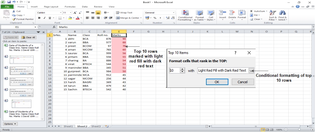
Chapter-9: Format only values that are above or below average - PK: An Excel Expert
Format Data Labels in Excel- Instructions - TeachUcomp, Inc. To format data labels in Excel, choose the set of data labels to format. To do this, click the "Format" tab within the "Chart Tools" contextual tab in the Ribbon. Then select the data labels to format from the "Chart Elements" drop-down in the "Current Selection" button group.
Formatting Worksheets in Excel 2010 - Computer Notes

Excel Conditional Formatting for 0 - Stack Overflow
Docs | How to use conditional formatting in Sheets

Conditionally formatting labels – learningtableaublog
Post a Comment for "39 conditional formatting data labels excel"