41 how to add data labels to a pie chart in excel on mac

› 2014/01/20 › excel-chart-titleHow to add titles to Excel charts in a minute. - Ablebits.com Jan 20, 2014 · In Excel 2013 the CHART TOOLS include 2 tabs: DESIGN and FORMAT. Click on the DESIGN tab. Open the drop-down menu named Add Chart Element in the Chart Layouts group. If you work in Excel 2010, go to the Labels group on the Layout tab. Choose 'Chart Title' and the position where you want your title to display. › 07 › 09Rotate charts in Excel - spin bar, column, pie and line charts Jul 09, 2014 · After being rotated my pie chart in Excel looks neat and well-arranged. Thus, you can see that it's quite easy to rotate an Excel chart to any angle till it looks the way you need. It's helpful for fine-tuning the layout of the labels or making the most important slices stand out. Rotate 3-D charts in Excel: spin pie, column, line and bar charts

Adding data labels to a pie chart - Excel General - OzGrid Free Excel ... Re: Adding data labels to a pie chart. Thanks again, norie. Really appreciate the help. I tried recording a macro while doing it manually (before my first post). But it didn't record anything about labels, much less making them bold.

How to add data labels to a pie chart in excel on mac

How To Add Text To A Pie Chart In Excel For Mac To display percentage values as labels on a pie chart. Add a pie chart to your report. For more information, see Add a Chart to a Report (Report Builder and SSRS). On the design surface, right-click on the pie and select Show Data Labels. The data labels should appear within each slice on the pie chart. How to Make a Pie Chart in Excel & Add Rich Data Labels to The Chart! Creating and formatting the Pie Chart. 1) Select the data. 2) Go to Insert> Charts> click on the drop-down arrow next to Pie Chart and under 2-D Pie, select the Pie Chart, shown below. 3) Chang the chart title to Breakdown of Errors Made During the Match, by clicking on it and typing the new title. Formatting data labels and printing pie charts on Excel for Mac 2019 ... Work around: Select the area of the chart - by selecting the cells behind where the chart is sitting > Print area> Select print area>File > print>then set print perameters (paper size, fit to page etc.) > Print. This worked. 2. When formatting data labels on an extended bar of pie chart: Excel does not allow me to:

How to add data labels to a pie chart in excel on mac. How Do I Add A Pie Chart In Excel For Mac - herevload Excel charts allow you to do a lot of customizations that help in representing the data in the best possible way. And one such example of customization is the ease with which you can add a secondary... How Do You Add Text To Pie Chart In Excel For Mac - needtree Where Is Dark Blue, Text 2 In Excel For Mac Snap An Image In Word Without Moving Text For Mac Mac Os X Syntax Highlighting For Rtf Rich Text Remove Background Color From Text Box In Word For Mac 2011 Plain Text For Mac How To Add Text Above A Table In Word For Mac Make Text Bigger In Outlook For Mac Calendar How to Make a Pie Chart in Excel - zembroe.norushcharge.com Add a name to the chart. To do so, click the B1 cell and then type in the chart's name.. For example, if you're making a chart about your budget, the B1 cell should say something like "2017 Budget".; You can also type in a clarifying label--e.g., "Budget Allocation"--in the A1 cell.A1 cell. How to display leader lines in pie chart in Excel? - ExtendOffice To display leader lines in pie chart, you just need to check an option then drag the labels out. 1. Click at the chart, and right click to select Format Data Labels from context menu. 2. In the popping Format Data Labels dialog/pane, check Show Leader Lines in the Label Options section. See screenshot:

› graphs › pie-chartsFree Pie Chart Maker - Make a Pie Chart in Canva Skip the complicated calculations – with Canva’s pie chart generator, you can turn raw data into a finished pie chart in minutes. A simple click will open the data section where you can add values. You can even copy and paste the data from a spreadsheet. Click the text to edit the labels. › Make-a-Pie-Chart-in-ExcelHow to Make a Pie Chart in Excel: 10 Steps (with Pictures) Apr 18, 2022 · Click the "Pie Chart" icon. This is a circular button in the "Charts" group of options, which is below and to the right of the Insert tab. You'll see several options appear in a drop-down menu: 2-D Pie - Create a simple pie chart that displays color-coded sections of your data. 3-D Pie - Uses a three-dimensional pie chart that displays color ... › charts › gauge-templateExcel Gauge Chart Template - Free Download - How to Create Step #7: Add the pointer data into the equation by creating the pie chart. Step #8: Realign the two charts. Step #9: Align the pie chart with the doughnut chart. Step #10: Hide all the slices of the pie chart except the pointer and remove the chart border. Step #11: Add the chart title and labels. How to Create and Format a Pie Chart in Excel - Lifewire To create a pie chart, highlight the data in cells A3 to B6 and follow these directions: On the ribbon, go to the Insert tab. Select Insert Pie Chart to display the available pie chart types. Hover over a chart type to read a description of the chart and to preview the pie chart. Choose a chart type.

How to Add Two Data Labels in Excel Chart (with Easy Steps) Step 4: Format Data Labels to Show Two Data Labels. Here, I will discuss a remarkable feature of Excel charts. You can easily show two parameters in the data label. For instance, you can show the number of units as well as categories in the data label. To do so, Select the data labels. Then right-click your mouse to bring the menu. How Do I Add A Pie Chart In Excel For Mac - coolnfile In this example, we have selected the first pie chart (called Pie) in the 2-D Pie section. Click Insert Insert Pie or Doughnut Chart, and then pick the chart you want. Click the chart and then click the icons next to the chart to add finishing touches: To show, hide, or format things like axis titles or data labels, click Chart Elements. EOF Create a chart in Excel for Mac - support.microsoft.com With the chart selected, click the Chart Design tab to do any of the following: Click Add Chart Element to modify details like the title, labels, and the legend. Click Quick Layout to choose from predefined sets of chart elements.

35 Data Label Excel - Labels For Your Ideas

How Do I Add A Pie Chart In Excel For Mac - lasopaluna Select first two columns of data, then in the Insert Tab from Ribbon, click Pie Chart. A basic pie chart will be created; Step 2: Delete Legend at the bottom (based on your setting, legend may appear in other position); Step 3: Add Data Labels to the pie chart: right click on the pie, then click 'Add Data Label'; The data labels were added to ...

29 Add Axis Label Excel Mac - 1000+ Labels Ideas

How to☝️Create a Pie of Pie Chart in Excel - SpreadsheetDaddy Start off by following the chart creation method as described below. Select your data. Navigate to the Insert menu. In the Chart submenu, click on Insert Pie or Doughnut Chart. Pick the Pie of Pie Chart type. Voila! With those few steps, you have added a Pie of Pie Chart to your worksheet.

34 How To Label Graphs In Excel - Labels Design Ideas 2020

How Do I Add A Pie Chart In Excel For Mac - revizionthat Nov 13, 2019 Add Data Labels to the Pie Chart. There are many different parts to a chart in Excel, such as the plot area that contains the pie chart representing the selected data series, the legend,...

How To Make A Cashier Count Chart In Excel : How to make an organizational chart - YouTube : Pie ...

support.microsoft.com › en-us › officeChange the format of data labels in a chart To get there, after adding your data labels, select the data label to format, and then click Chart Elements > Data Labels > More Options. To go to the appropriate area, click one of the four icons ( Fill & Line , Effects , Size & Properties ( Layout & Properties in Outlook or Word), or Label Options ) shown here.

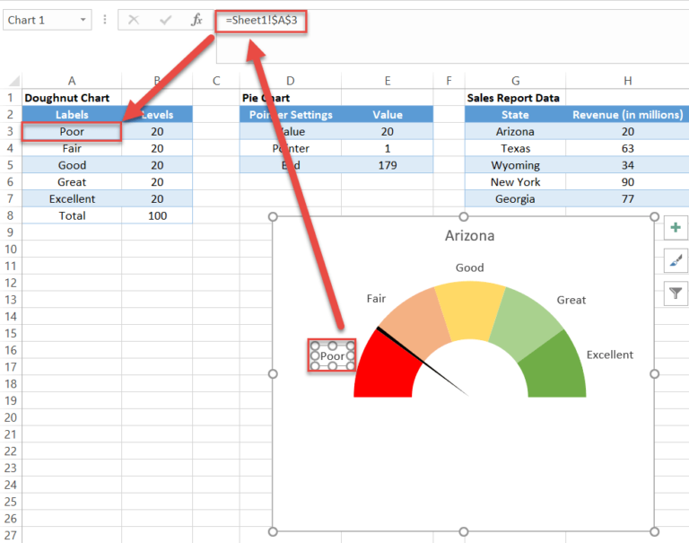
Excel Gauge Chart Template - Free Download - How to Create

Pie Chart in Excel | How to Create Pie Chart - EDUCBA Step 1: Do not select the data; rather, place a cursor outside the data and insert one PIE CHART. Go to the Insert tab and click on a PIE. Step 2: once you click on a 2-D Pie chart, it will insert the blank chart as shown in the below image. Step 3: Right-click on the chart and choose Select Data. Step 4: once you click on Select Data, it will ...

31 How To Label Vertical Axis In Excel

How Do I Add A Pie Chart In Excel For Mac - panlasopa To format a data table, go to the Format tab and click the table data in the chart. With the chart selected, click the Chart Design tab to do any of the following: Click Add Chart Element to modify details like the title, labels, and the legend. Click Quick Layout to choose from predefined sets of chart elements.

31 How To Label Vertical Axis In Excel

support.microsoft.com › en-us › officeAdd or remove data labels in a chart - support.microsoft.com For example, in the pie chart below, without the data labels it would be difficult to tell that coffee was 38% of total sales. Depending on what you want to highlight on a chart, you can add labels to one series, all the series (the whole chart), or one data point. Add data labels. You can add data labels to show the data point values from the ...

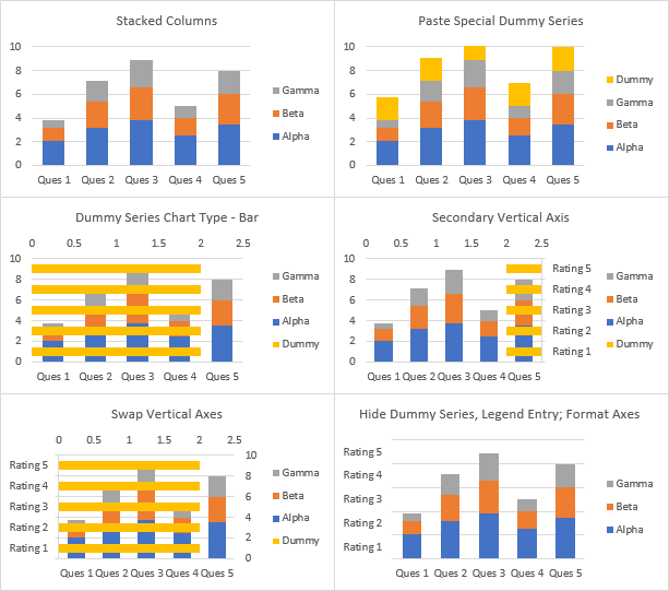
New Charts in Excel 2016 • My Online Training Hub

Formatting data labels and printing pie charts on Excel for Mac 2019 ... Work around: Select the area of the chart - by selecting the cells behind where the chart is sitting > Print area> Select print area>File > print>then set print perameters (paper size, fit to page etc.) > Print. This worked. 2. When formatting data labels on an extended bar of pie chart: Excel does not allow me to:

Share :